Chapter 1 Introduction to Loss Data Analytics

This file contains illustrative R code for computing analysis on the Property Fund data. When reviewing this code,you should open an R session, copy-and-paste the code, and see it perform. Then, you will be able to change parameters, look up commands, and so forth, as you go.This code uses the dataset PropertyFundInsample.csv

1.1 Read in Property Fund Data

Insample <- read.csv("Data/PropertyFundInsample.csv", header=T, na.strings=c("."), stringsAsFactors=FALSE)
Insample2010 <- subset(Insample, Year==2010)

A few quick notes on these commands:

• read.csv reads a csv file and creates data frame from it, with cases corresponding to rows and variables to columns in the file.

• The assignment operator <- is analogous to an equal sign in mathematics. The command Insample <- read.csv("PropertyFundInsample.csv", header=T, na.strings=c("."), stringsAsFactors=FALSE) means we give the name Insample to the data read.

• The subset() function is used to select variables and observations. In this illustration, we selected observations from year 2010.

1.2 Claim Frequency Distribution

In 2010 there were 1,110 policyholders in the property fund. Table 1.1 shows the distribution of the 1,377 claims.

1.2.1 Property fund distribution for 2010

Table 1.1

library(pander)
Table<-as.data.frame(table(Insample2010$Freq))
names(Table)<-c("Number of Claims", "Frequncy")
pander(t(Table))

Number of Claims	0	1	2	3	4	5	6	7	8	9	10	11	13	14	15	16	17	18	19	30	39	103	239
Frequncy	707	209	86	40	18	12	9	4	6	1	3	2	1	2	1	2	1	1	1	1	1	1	1

The average number of claims for this sample was 1.24 (=1377/1110). See table 1.2 below.

Table 1.2

pander(summary(Insample2010$Freq))

Min.	1st Qu.	Median	Mean	3rd Qu.	Max.
0	0	0	1.241	1	239

A few quick notes on these commands:

• Many useful R functions come in packages and to use these functions you have to install them. One way to install a package is by using the command line install.packages("<the package's name>") . In addition, to read more about a function you use the command help("function name") .

• The pander function is used here to create nicer tables than regular R output. To use this function you need to download the pander package. For the normal R output in the illustration above, use the command line summary(Insample2010$Freq).

• The names() function is used to to get or assign names of an object . In this illustration, we assigned Number of Claims and Frequency to the two columns in the data frame .

• The t() function is used to transpose a dataframe or a matrix.

1.3 Average Severity Distribution for 2010

Table 1.3 summarizes the sample distribution of average severity from the 403 policyholders; Figure 1.2 provides further information about the distribution of sample claims, showing a distribution that is dominated by this single large claim so that the histogram is not very helpful. Even when removing the large claim, you will find a distribution that is skewed to the right. A generally accepted technique is to work with claims in logarithmic units especially for graphical purposes; the corresponding figure in the right-hand panel is much easier to interpret.

Table 1.3

InsamplePos2010 <- subset(Insample2010, yAvg>0)
pander(summary(InsamplePos2010$yAvg))

Min.	1st Qu.	Median	Mean	3rd Qu.	Max.
166.7	2226	4951	56330	11900	12920000

length(InsamplePos2010$yAvg)

## [1] 403

Note: The length() function sets the length of a vector (list) or other objects.

1.3.1 Plot of average claims

Figure 1.2

par(mfrow=c(1, 2))
hist(InsamplePos2010$yAvg, main="", xlab="Average Claims")
hist(log(InsamplePos2010$yAvg), main="", xlab="Logarithmic Average Claims")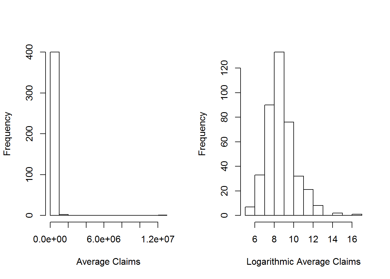

A few quick notes on these commands:

• The par(mfrow) function is handy for creating a simple multi-paneled plot. mfrow is a vector of length 2, where the first argument specifies the number of rows and the second the number of columns of plots.

• The hist() computes a histogram of the given data values. You put the name of your dataset in between the parentheses of this function

1.4 Rating Variables

Earlier we considered a sample of 1,110 observations which may seem like a lot. However, as we will seen in our forthcoming applications, because of the preponderance of zeros and the skewed nature of claims, actuaries typically yearn for more data. One common approach that we adopt here is to examine outcomes from multiple years, thus increasing the sample size.

Table 1.4 shows that the average claim varies over time.

1.4.1 Average claims over time

Table 1.4

library(doBy)
T1A <- summaryBy(Freq ~ Year, data = Insample,   
                 FUN = function(x) { c(m = mean(x), num=length(x)) } )
T1B <- summaryBy(yAvg    ~ Year, data = Insample,   
                 FUN = function(x) { c(m = mean(x), num=length(x)) } )
T1C <- summaryBy(BCcov    ~ Year, data = Insample,   
                 FUN = function(x) { c(m = mean(x), num=length(x)) } )
Table1In <- cbind(T1A[1],T1A[2],T1B[2],T1C[2],T1A[3])
names(Table1In) <- c("Year", "Average Freq","Average Sev", "Average Coverage","No. of Policyholders")
pander(Table1In)

Year	Average Freq	Average Sev	Average Coverage	No. of Policyholders
2006	0.9515	9695	32498186	1154
2007	1.167	6544	35275949	1138
2008	0.9742	5311	37267485	1125
2009	1.219	4572	40355382	1112
2010	1.241	20452	41242070	1110

A few quick notes on these commands:

• The summaryBy() function provides summary statistics of a variable across different groups. You need to install the doBy package to use the command.

• The cbind() combines vector, matrix or data frame by columns. The row number of the two datasets must be equal.

• The c() function combines its arguments to form a vector.

For a different look at this five-year sample, Table 1.5 summarizes the distribution of our two outcomes, frequency and claims amount. In each case, the average exceeds the median, suggesting that the distributions are right-skewed.

1.4.2 Frequency and claims statistics of full data

Table 1.5

t1<- summaryBy(Insample$Freq ~ 1, data = Insample, 
                 FUN = function(x) { c(ma=min(x), m1=median(x),m=mean(x),mb=max(x)) } )
names(t1) <- c("Minimum", "Median","Average", "Maximum")
t2 <- summaryBy(Insample$yAvg ~ 1, data = Insample, 
                 FUN = function(x) { c(ma=min(x), m1=median(x), m=mean(x),mb=max(x)) } )
names(t2) <- c("Minimum", "Median","Average", "Maximum")
t3 <- summaryBy(Deduct ~ 1, data = Insample, 
                 FUN = function(x) { c(ma=min(x), m1=median(x), m=mean(x),mb=max(x)) } )
names(t3) <- c("Minimum", "Median","Average", "Maximum")
t4 <- summaryBy(BCcov/1000 ~ 1, data = Insample, 
                 FUN = function(x) { c(ma=min(x), m1=median(x), m=mean(x),mb=max(x)) } )
names(t4) <- c("Minimum", "Median","Average", "Maximum")
Table2 <- rbind(t1,t2,t3,t4)
Table2a <- round(Table2,3)
Rowlable <- rbind("Claim Frequency","Claim Severity","Deductible","Coverage (000's)")
Table2aa <- cbind(Rowlable,as.matrix(Table2a))
pander(Table2aa)

	Minimum	Median	Average	Maximum
Claim Frequency	0	0	1.109	263
Claim Severity	0	0	9291.565	12922217.84
Deductible	500	1000	3364.87	1e+05
Coverage (000’s)	8.937	11353.566	37280.855	2444796.98

A few quick notes on these commands:

• The rbind() combines vector, matrix or data frame by rows. The column of the two datasets must be same.

• The round() function rounds the values in its first argument to the specified number of decimal places (default 0).

Table 1.6 describes the rating variables considered in this chapter. To handle the skewness, we henceforth focus on logarithmic transformations of coverage and deductibles. To get a sense of the relationship between the non-continuous rating variables and claims, Table 1.7 relates the claims outcomes to these categorical variables.

1.4.3 Rating variable description

See table 1.6 below for variables and variable description.

Table 1.6

R code for table 1.6

---

des <- read.table(header=TRUE, text='
 Variable Description
  "BCcov"  "Total building and content coverage in dollars"
  "Deduct"  "Deductible in dollars"
"Entity Type"   "Categorical variable that is one of six types: (Village, City, County, Misc, School, or Town)"
"AlarmCredit"   "Categorical variable that is one of four types: (0%, 5%, 10%, or 15%), for automatic smoke alarms in main rooms"
"NoClaimCredit" "Binary variable to indicate no claims in the past two years"
"Fire5" "Binary variable to indicate the fire class is below 5. (The range of fire class is 0~10)" ')

---

pander(des)

Variable	Description
BCcov	Total building and content coverage in dollars
Deduct	Deductible in dollars
Entity Type	Categorical variable that is one of six types: (Village, City, County, Misc, School, or Town)
AlarmCredit	Categorical variable that is one of four types: (0%, 5%, 10%, or 15%), for automatic smoke alarms in main rooms
NoClaimCredit	Binary variable to indicate no claims in the past two years
Fire5	Binary variable to indicate the fire class is below 5. (The range of fire class is 0~10)

1.4.4 Frequency and claims by rating variables

Table 1.7 shows claims summary by Entity Type, Fire Class, and No Claim Credit.

Table 1.7: R code for table 1.7

---

# Table 1.7
ByVarSumm<-function(datasub){
  tempA <- summaryBy(Freq    ~ 1 , data = datasub,   
                     FUN = function(x) { c(m = mean(x), num=length(x)) } )
  datasub1<-  subset(datasub, yAvg>0)
  tempB <- summaryBy(yAvg   ~ 1, data = datasub1,
                     FUN = function(x) { c(m = mean(x)) } )
  tempC <- merge(tempA,tempB,all.x=T)[c(2,1,3)]
  tempC1 <- as.matrix(tempC)
  return(tempC1)
}

datasub <-  subset(Insample, TypeVillage == 1);   
t1 <- ByVarSumm(datasub)
datasub <-  subset(Insample, TypeCity == 1);      
t2 <- ByVarSumm(datasub)
datasub <-  subset(Insample, TypeCounty == 1);   
t3 <- ByVarSumm(datasub)
datasub <-  subset(Insample, TypeMisc == 1);      
t4 <- ByVarSumm(datasub)
datasub <-  subset(Insample, TypeSchool == 1);    
t5 <- ByVarSumm(datasub)
datasub <-  subset(Insample, TypeTown == 1);      
t6 <- ByVarSumm(datasub)
datasub <-  subset(Insample, Fire5 == 0);                      
t7 <- ByVarSumm(datasub)
datasub <-  subset(Insample, Fire5 == 1);                      
t8 <- ByVarSumm(datasub)
datasub <-  subset(Insample, Insample$NoClaimCredit == 0);
t9 <- ByVarSumm(datasub)
datasub <-  subset(Insample, Insample$NoClaimCredit == 1);
t10 <- ByVarSumm(datasub)
t11 <- ByVarSumm(Insample)

Tablea <- rbind(t1,t2,t3,t4,t5,t6,t7,t8,t9,t10,t11)
Tableaa <- round(Tablea,3)
Rowlable <- rbind("Village","City","County","Misc","School",
                  "Town","Fire5--No","Fire5--Yes","NoClaimCredit--No",
                  "NoClaimCredit--Yes","Total")
Table4 <- cbind(Rowlable,as.matrix(Tableaa))

---

pander(Table4)

	Freq.num	Freq.m	yAvg.m
Village	1341	0.452	10645.206
City	793	1.941	16924.035
County	328	4.899	15453.206
Misc	609	0.186	43036.076
School	1597	1.434	64346.394
Town	971	0.103	19831.048
Fire5–No	2508	0.502	13935.421
Fire5–Yes	3131	1.596	41421.263
NoClaimCredit–No	3786	1.501	31365.085
NoClaimCredit–Yes	1853	0.31	30498.714
Total	5639	1.109	31206.155

Table 1.8 shows claims summary by Entity Type and Alarm Credit

Table 1.8:

R code for table 1.8

---

ByVarSumm<-function(datasub){
  tempA <- summaryBy(Freq    ~ AC00 , data = datasub,   
                     FUN = function(x) { c(m = mean(x), num=length(x)) } )
  datasub1 <-  subset(datasub, yAvg>0)
  if(nrow(datasub1)==0) { n<-nrow(datasub)
    return(c(0,0,n))
  } else 
  {
    tempB <- summaryBy(yAvg   ~ AC00, data = datasub1,
                       FUN = function(x) { c(m = mean(x)) } )
    tempC <- merge(tempA,tempB,all.x=T)[c(2,4,3)]
    tempC1 <- as.matrix(tempC)
    return(tempC1)
  }
}
AlarmC <- 1*(Insample$AC00==1) + 2*(Insample$AC05==1)+ 3*(Insample$AC10==1)+ 4*(Insample$AC15==1)
ByVarCredit<-function(ACnum){
datasub <-  subset(Insample, TypeVillage == 1 & AlarmC == ACnum); 
  t1 <- ByVarSumm(datasub)
datasub <-  subset(Insample, TypeCity == 1 & AlarmC == ACnum);      
  t2 <- ByVarSumm(datasub)
datasub <-  subset(Insample, TypeCounty == 1 & AlarmC == ACnum);   
  t3 <- ByVarSumm(datasub)
datasub <-  subset(Insample, TypeMisc == 1 & AlarmC == ACnum);
  t4 <- ByVarSumm(datasub)
datasub <-  subset(Insample, TypeSchool == 1 & AlarmC == ACnum);    
  t5 <- ByVarSumm(datasub)
datasub <-  subset(Insample, TypeTown == 1 & AlarmC ==ACnum);      
  t6 <- ByVarSumm(datasub)
datasub <-  subset(Insample, AlarmC == ACnum);  
  t7 <- ByVarSumm(datasub)
Tablea <- rbind(t1,t2,t3,t4,t5,t6,t7)
Tableaa <- round(Tablea,3)
Rowlable <- rbind("Village","City","County","Misc","School",
                  "Town","Total")
Table4 <- cbind(Rowlable,as.matrix(Tableaa))
}
Table4a <- ByVarCredit(1)    #Claims Summary by Entity Type and Alarm Credit==00
Table4b <- ByVarCredit(2)    #Claims Summary by Entity Type and Alarm Credit==05 
Table4c <- ByVarCredit(3)    #Claims Summary by Entity Type and Alarm Credit==10
Table4d <- ByVarCredit(4)    #Claims Summary by Entity Type and Alarm Credit==15

---

pander(Table4a) #Claims Summary by Entity Type and Alarm Credit==00

	Freq.m	yAvg.m	Freq.num
Village	0.326	11077.997	829
City	0.893	7575.979	244
County	2.14	16012.719	50
Misc	0.117	15122.127	386
School	0.422	25522.708	294
Town	0.083	25257.084	808
Total	0.318	15118.491	2611

pander(Table4b) #Claims Summary by Entity Type and Alarm Credit==05 

		Freq.m	yAvg.m	Freq.num
	Village	0.278	8086.057	54
	City	2.077	4150.125	13
t3	County	0	0	1
	Misc	0.278	13063.933	18
	School	0.41	14575.003	122
	Town	0.194	3937.29	31
	Total	0.431	10762.112	239

pander(Table4c) #Claims Summary by Entity Type and Alarm Credit==10

	Freq.m	yAvg.m	Freq.num
Village	0.5	8792.376	50
City	1.258	8625.169	31
County	2.125	11687.969	8
Misc	0.077	3923.375	26
School	0.488	11596.912	168
Town	0.091	2338.06	44
Total	0.517	10194.094	327

pander(Table4d) #Claims Summary by Entity Type and Alarm Credit==15

	Freq.m	yAvg.m	Freq.num
Village	0.725	10543.752	408
City	2.485	20469.514	505
County	5.513	15475.74	269
Misc	0.341	87020.878	179
School	2.008	85139.974	1013
Town	0.261	9489.613	88
Total	2.093	41458.312	2462