Chapter 4 Model Selection and Inference

This file contains illustrative R code for computing important count distributions. When reviewing this code, you should open an R session, copy-and-paste the code, and see it perform. Then, you will be able to change parameters, look up commands, and so forth, as you go.This code uses the dataset CLAIMLEVEL.csv

4.1 Claim level data of Property Fund

This section summarizes claims from the property fund for year 2010 and plots the data.

## Read in data and get number of claims.  
ClaimLev <- read.csv("Data/CLAIMLEVEL.csv", header=TRUE); nrow(ClaimLev); # 6258

## [1] 6258

#2010 subset 
ClaimData<-subset(ClaimLev,Year==2010); 
length(unique(ClaimData$PolicyNum))        #403 unique policyholders

## [1] 403

NTot = nrow(ClaimData)                     #1377 individual claims
NTot

## [1] 1377

# As an alternative, you can simulate Claims
#NTot = 13770
#alphahat = 2
#thetahat =  100

#Claim = rgamma(NTot, shape = alphahat, scale = thetahat)
#Claim = rparetoII(NTot, loc = 0,  shape = alphahat, scale = thetahat)
# GB2
#Claim = thetahat*rgamma(NTot, shape = alphahat, scale = 1)/rgamma(NTot, shape = 1, scale =1) 
#ClaimData <- data.frame(Claim)

###################################################

4.1.1 Summary of claims

The output below provides summary on claims data for 2010 and summary in logarithmic units.

# Summarizing the claim data for 2010
summary(ClaimData$Claim);     sd(ClaimData$Claim)

##     Min.  1st Qu.   Median     Mean  3rd Qu.     Max. 
##        1      788     2250    26620     6171 12920000

## [1] 368029.7

# Summarizing logarithmic claims for 2010
summary(log(ClaimData$Claim));sd(log(ClaimData$Claim))

##    Min. 1st Qu.  Median    Mean 3rd Qu.    Max. 
##   0.000   6.670   7.719   7.804   8.728  16.370

## [1] 1.683297

4.1.2 Plot of claims

The plots below provides further information about the distribution of sample claims.

#histogram 
par(mfrow=c(1, 2))
hist(ClaimData$Claim, main="", xlab="Claims")
hist(log(ClaimData$Claim), main="", xlab="Logarithmic Claims")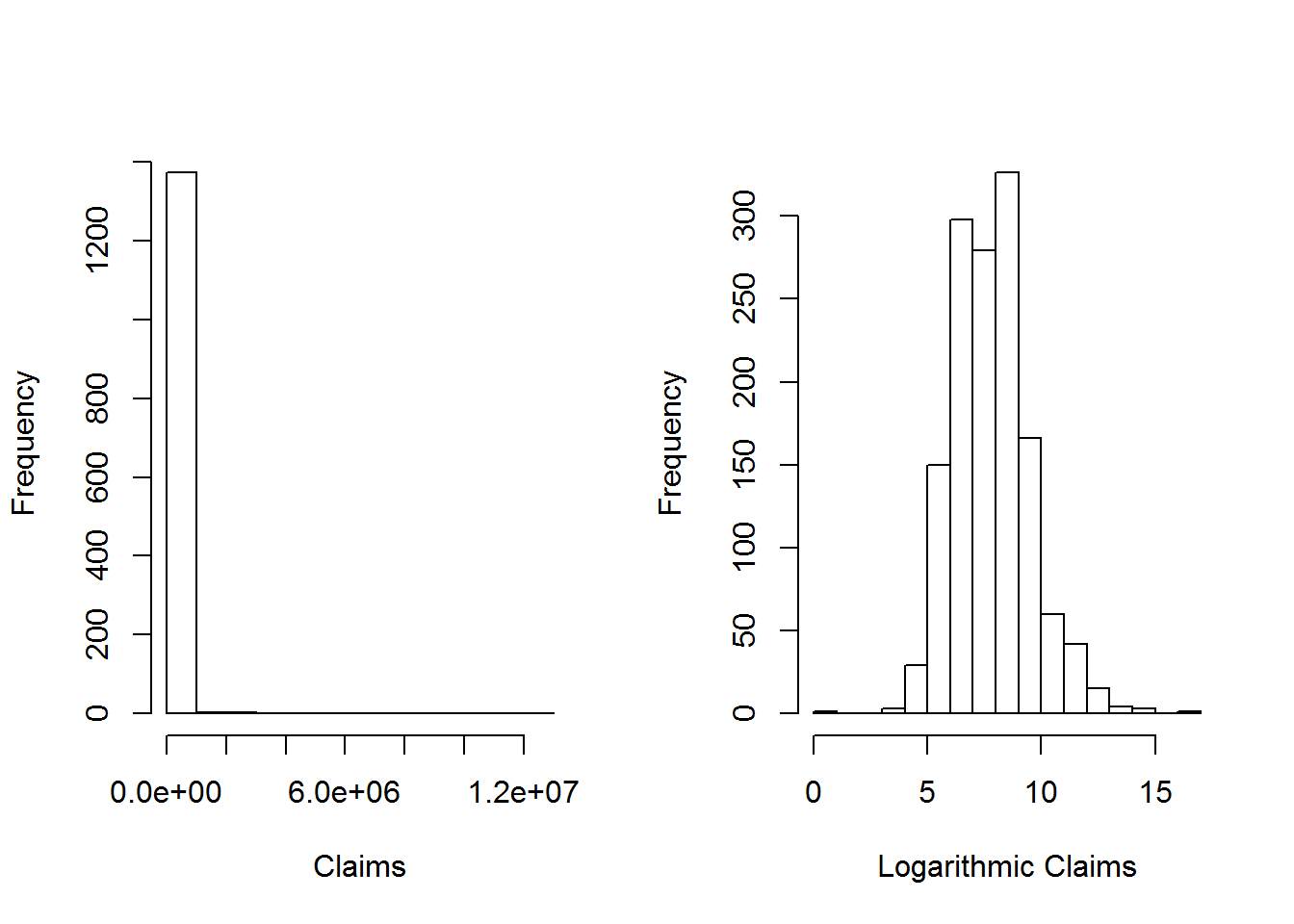

#dev.off()

4.2 Fitting distributions

This section shows how to fit basic distributions to a data set.

4.2.1 Inference assuming a lognormal distribution

The results below assume that the data follow a lognormal distribution and usesVGAM library for estimation of parameters

#  Inference assuming a lognormal distribution
#  First, take the log of the data and assume normality
y = log(ClaimData$Claim)
summary(y);sd(y)

##    Min. 1st Qu.  Median    Mean 3rd Qu.    Max. 
##   0.000   6.670   7.719   7.804   8.728  16.370

## [1] 1.683297

# confidence intervals and hypothesis test
t.test(y,mu=log(5000))   # H0: mu_o=log(5000)=8.517

## 
##  One Sample t-test
## 
## data:  y
## t = -15.717, df = 1376, p-value < 2.2e-16
## alternative hypothesis: true mean is not equal to 8.517193
## 95 percent confidence interval:
##  7.715235 7.893208
## sample estimates:
## mean of x 
##  7.804222

#mean of the lognormal distribution
exp(mean(y)+sd(y)^2/2)

## [1] 10106.82

mean(ClaimData$Claim)

## [1] 26622.59

#Alternatively, assume that the data follow a lognormal distribution
#Use "VGAM" library for estimation of parameters 
library(VGAM)
fit.LN <- vglm(Claim ~ 1, family=lognormal, data = ClaimData)
summary(fit.LN)

## 
## Call:
## vglm(formula = Claim ~ 1, family = lognormal, data = ClaimData)
## 
## 
## Pearson residuals:
##                 Min      1Q   Median     3Q    Max
## meanlog     -4.6380 -0.6740 -0.05083 0.5487  5.093
## loge(sdlog) -0.7071 -0.6472 -0.44003 0.1135 17.636
## 
## Coefficients: 
##               Estimate Std. Error z value Pr(>|z|)    
## (Intercept):1  7.80422    0.04535  172.10   <2e-16 ***
## (Intercept):2  0.52039    0.01906   27.31   <2e-16 ***
## ---
## Signif. codes:  0 '***' 0.001 '**' 0.01 '*' 0.05 '.' 0.1 ' ' 1
## 
## Number of linear predictors:  2 
## 
## Names of linear predictors: meanlog, loge(sdlog)
## 
## Log-likelihood: -13416.87 on 2752 degrees of freedom
## 
## Number of iterations: 3

coef(fit.LN)                 # coefficients

## (Intercept):1 (Intercept):2 
##     7.8042218     0.5203908

confint(fit.LN, level=0.95)  # confidence intervals for model parameters

##                   2.5 %    97.5 %
## (Intercept):1 7.7153457 7.8930978
## (Intercept):2 0.4830429 0.5577387

logLik(fit.LN)               #loglikelihood for lognormal

## [1] -13416.87

AIC(fit.LN)                  #AIC for lognormal

## [1] 26837.74

BIC(fit.LN)                  #BIC for lognormal

## [1] 26848.2

vcov(fit.LN)                 # covariance matrix for model parameters

##               (Intercept):1 (Intercept):2
## (Intercept):1   0.002056237  0.0000000000
## (Intercept):2   0.000000000  0.0003631082

#mean of the lognormal distribution
exp(mean(y)+sd(y)^2/2)

## [1] 10106.82

exp(coef(fit.LN))

## (Intercept):1 (Intercept):2 
##   2450.927448      1.682685

A few quick notes on these commands:

The t.test() function can be used for a variety of t-tests. In this illustration, it was used to test $H_0=\mu_0=\log(5000)=8.517$
The vglm() function is used to fit vector generalized linear models (VGLMs). See help(vglm) for other modeling options.
The coef() function returns the estimated coefficients from the vglm or other modeling functions.
The confint function provides the confidence intervals for model parameters.
The loglik function provides the log-likelihood value for the lognormal estimation from the vglm or other modeling functions.
AIC() and BIC() returns Akaike’s Information Criterion and BIC or SBC (Schwarz’s Bayesian criterion) for the fitted lognormal model. $\text{AIC} =-2* \text{(loglikelihood)} + 2*\text{npar}$ , where npar represents the number of parameters in the fitted model, and $\text{BIC} =-2* \text{log-likelihood} + \log(n)* \text{npar}$ where $n$ is the number of observations.
vcov() returns the covariance matrix for model parameters

4.2.2 Inference assuming a gamma distribution

The results below assume that the data follow a Gamma distribution and usesVGAM library for estimation of parameters.

#  Inference assuming a gamma distribution
#install.packages("VGAM")
library(VGAM)
fit.gamma <- vglm(Claim ~ 1, family=gamma2, data = ClaimData)
summary(fit.gamma)

## 
## Call:
## vglm(formula = Claim ~ 1, family = gamma2, data = ClaimData)
## 
## 
## Pearson residuals:
##                  Min      1Q  Median      3Q     Max
## loge(mu)      -0.539 -0.5231 -0.4935 -0.4141 261.117
## loge(shape) -153.990 -0.1024  0.2335  0.4969   0.772
## 
## Coefficients: 
##               Estimate Std. Error z value Pr(>|z|)    
## (Intercept):1 10.18952    0.04999  203.82   <2e-16 ***
## (Intercept):2 -1.23582    0.03001  -41.17   <2e-16 ***
## ---
## Signif. codes:  0 '***' 0.001 '**' 0.01 '*' 0.05 '.' 0.1 ' ' 1
## 
## Number of linear predictors:  2 
## 
## Names of linear predictors: loge(mu), loge(shape)
## 
## Log-likelihood: -14150.59 on 2752 degrees of freedom
## 
## Number of iterations: 13

coef(fit.gamma)                 # This uses a different parameterization

## (Intercept):1 (Intercept):2 
##     10.189515     -1.235822

(theta<-exp(coef(fit.gamma)[1])/exp(coef(fit.gamma)[2])) #theta=mu/alpha

## (Intercept):1 
##      91613.78

(alpha<-exp(coef(fit.gamma)[2]))

## (Intercept):2 
##     0.2905959

plot(density(log(ClaimData$Claim)), main="", xlab="Log Expenditures")
x <- seq(0,15,by=0.01)
fgamma_ex = dgamma(exp(x), shape = alpha, scale=theta)*exp(x)
lines(x,fgamma_ex,col="blue")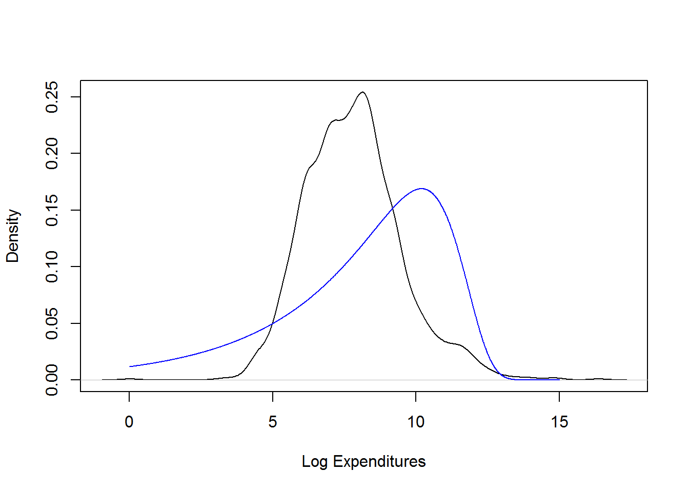

confint(fit.gamma, level=0.95)  # confidence intervals for model parameters

##                   2.5 %    97.5 %
## (Intercept):1 10.091533 10.287498
## (Intercept):2 -1.294648 -1.176995

logLik(fit.gamma)               #loglikelihood for gamma

## [1] -14150.59

AIC(fit.gamma)                  #AIC for gamma

## [1] 28305.17

BIC(fit.gamma)                  #BIC for gamma

## [1] 28315.63

vcov(fit.gamma)                 # covariance matrix for model parameters

##               (Intercept):1 (Intercept):2
## (Intercept):1   0.002499196  0.0000000000
## (Intercept):2   0.000000000  0.0009008397

# Here is a check on the formulas
#AIC using formula : -2*(loglik)+2(number of parameters)
-2*(logLik(fit.gamma))+2*(length(coef(fit.gamma)))

## [1] 28305.17

#BIC using formula : -2*(loglik)+(number of parameters)*(log(n))
-2*(logLik(fit.gamma))+length(coef(fit.gamma, matrix = TRUE))*log(nrow(ClaimData))

## [1] 28315.63

#Alternatively, we could a gamma distribution using glm
library(MASS)
fit.gamma2 <- glm(Claim~1, data=ClaimData,family=Gamma(link=log)) 
summary(fit.gamma2, dispersion = gamma.dispersion(fit.gamma2))

## 
## Call:
## glm(formula = Claim ~ 1, family = Gamma(link = log), data = ClaimData)
## 
## Deviance Residuals: 
##    Min      1Q  Median      3Q     Max  
## -4.287  -2.258  -1.764  -1.178  30.926  
## 
## Coefficients:
##             Estimate Std. Error z value Pr(>|z|)    
## (Intercept) 10.18952    0.04999   203.8   <2e-16 ***
## ---
## Signif. codes:  0 '***' 0.001 '**' 0.01 '*' 0.05 '.' 0.1 ' ' 1
## 
## (Dispersion parameter for Gamma family taken to be 3.441204)
## 
##     Null deviance: 6569.1  on 1376  degrees of freedom
## Residual deviance: 6569.1  on 1376  degrees of freedom
## AIC: 28414
## 
## Number of Fisher Scoring iterations: 14

(theta<-exp(coef(fit.gamma2))*gamma.dispersion(fit.gamma2)) #theta=mu/alpha

## (Intercept) 
##    91613.78

(alpha<-1/gamma.dispersion(fit.gamma2) )

## [1] 0.2905959

logLik(fit.gamma2)  #log - likelihood slightly different from vglm

## 'log Lik.' -14204.77 (df=2)

AIC(fit.gamma2)     #AIC

## [1] 28413.53

BIC(fit.gamma2)     #BIC

## [1] 28423.99

Note : The output from coef(fit.gamma) uses the parameterization $\mu=\theta * \alpha$ . coef(fit.gamma)[1]= $\log(\mu)$ and coef(fit.gamma)[2]= $\log(\alpha)$ ,which implies , $\alpha$ =exp(coef(fit.gamma)[2]) and $\theta=\mu/\alpha$ =exp(coef(fit.gamma)[1])/exp(coef(fit.gamma)[2])

4.2.3 Inference assuming a Pareto Distribution

The results below assume that the data follow a Pareto distribution and usesVGAM library for estimation of parameters.

fit.pareto <- vglm(Claim ~ 1, paretoII, loc=0, data = ClaimData)
summary(fit.pareto)

## 
## Call:
## vglm(formula = Claim ~ 1, family = paretoII, data = ClaimData, 
##     loc = 0)
## 
## 
## Pearson residuals:
##                 Min      1Q Median     3Q   Max
## loge(scale)  -6.332 -0.8289 0.1875 0.8832 1.174
## loge(shape) -10.638  0.0946 0.4047 0.4842 0.513
## 
## Coefficients: 
##                 Estimate Std. Error z value Pr(>|z|)    
## (Intercept):1  7.7329210  0.0933332  82.853   <2e-16 ***
## (Intercept):2 -0.0008753  0.0538642  -0.016    0.987    
## ---
## Signif. codes:  0 '***' 0.001 '**' 0.01 '*' 0.05 '.' 0.1 ' ' 1
## 
## Number of linear predictors:  2 
## 
## Names of linear predictors: loge(scale), loge(shape)
## 
## Log-likelihood: -13404.64 on 2752 degrees of freedom
## 
## Number of iterations: 5

head(fitted(fit.pareto))

##         [,1]
## [1,] 2285.03
## [2,] 2285.03
## [3,] 2285.03
## [4,] 2285.03
## [5,] 2285.03
## [6,] 2285.03

coef(fit.pareto)

## (Intercept):1 (Intercept):2 
##  7.7329210483 -0.0008752515

exp(coef(fit.pareto))

## (Intercept):1 (Intercept):2 
##  2282.2590626     0.9991251

confint(fit.pareto, level=0.95)  # confidence intervals for model parameters

##                    2.5 %    97.5 %
## (Intercept):1  7.5499914 7.9158507
## (Intercept):2 -0.1064471 0.1046966

logLik(fit.pareto)               #loglikelihood for pareto

## [1] -13404.64

AIC(fit.pareto)                  #AIC for pareto

## [1] 26813.29

BIC(fit.pareto)                  #BIC for pareto

## [1] 26823.74

vcov(fit.pareto)                 # covariance matrix for model parameters

##               (Intercept):1 (Intercept):2
## (Intercept):1   0.008711083   0.004352904
## (Intercept):2   0.004352904   0.002901350

4.2.4 Inference assuming an exponential distribution

The results below assume that the data follow an exponential distribution and usesVGAM library for estimation of parameters.

fit.exp <- vglm(Claim ~ 1, exponential, data = ClaimData)
summary(fit.exp)

## 
## Call:
## vglm(formula = Claim ~ 1, family = exponential, data = ClaimData)
## 
## 
## Pearson residuals:
##               Min     1Q Median     3Q Max
## loge(rate) -484.4 0.7682 0.9155 0.9704   1
## 
## Coefficients: 
##              Estimate Std. Error z value Pr(>|z|)    
## (Intercept) -10.18952    0.02695  -378.1   <2e-16 ***
## ---
## Signif. codes:  0 '***' 0.001 '**' 0.01 '*' 0.05 '.' 0.1 ' ' 1
## 
## Number of linear predictors:  1 
## 
## Name of linear predictor: loge(rate) 
## 
## Residual deviance: 6569.099 on 1376 degrees of freedom
## 
## Log-likelihood: -15407.96 on 1376 degrees of freedom
## 
## Number of iterations: 6

(theta = 1/exp(coef(fit.exp)))

## (Intercept) 
##    26622.59

# Can also fit using the "glm" package
fit.exp2 <- glm(Claim~1, data=ClaimData,family=Gamma(link=log)) 
summary(fit.exp2,dispersion=1)

## 
## Call:
## glm(formula = Claim ~ 1, family = Gamma(link = log), data = ClaimData)
## 
## Deviance Residuals: 
##    Min      1Q  Median      3Q     Max  
## -4.287  -2.258  -1.764  -1.178  30.926  
## 
## Coefficients:
##             Estimate Std. Error z value Pr(>|z|)    
## (Intercept) 10.18952    0.02695   378.1   <2e-16 ***
## ---
## Signif. codes:  0 '***' 0.001 '**' 0.01 '*' 0.05 '.' 0.1 ' ' 1
## 
## (Dispersion parameter for Gamma family taken to be 1)
## 
##     Null deviance: 6569.1  on 1376  degrees of freedom
## Residual deviance: 6569.1  on 1376  degrees of freedom
## AIC: 28414
## 
## Number of Fisher Scoring iterations: 14

(theta<-exp(coef(fit.exp2)))

## (Intercept) 
##    26622.59

4.2.5 Inference assuming an exponential distribution

The results below assume that the data follow a GB2 distribution and uses the maximum likelihood technique for parameter estimation.

#  Inference assuming a GB2 Distribution - this is more complicated
# The likelihood functon of GB2 distribution (negative for optimization)
likgb2 <- function(param) {
  a1 <- param[1]
  a2 <- param[2]
  mu <- param[3]
  sigma <- param[4]
  yt <- (log(ClaimData$Claim)-mu)/sigma
  logexpyt<-ifelse(yt>23,yt,log(1+exp(yt)))
  logdens <- a1*yt - log(sigma) - log(beta(a1,a2)) - (a1+a2)*logexpyt -log(ClaimData$Claim) 
  return(-sum(logdens))
}
#  "optim" is a general purpose minimization function
gb2bop <- optim(c(1,1,0,1),likgb2,method=c("L-BFGS-B"),
                lower=c(0.01,0.01,-500,0.01),upper=c(500,500,500,500),hessian=TRUE)

#Estimates
gb2bop$par

## [1] 2.830928 1.202500 6.328981 1.294552

#standard error
sqrt(diag(solve(gb2bop$hessian)))

## [1] 0.9997743 0.2918469 0.3901929 0.2190362

#t-statistics
(tstat = gb2bop$par/sqrt(diag(solve(gb2bop$hessian))) )

## [1]  2.831567  4.120313 16.220133  5.910217

# density for GB II
gb2density <- function(x){
  a1 <- gb2bop$par[1]
  a2 <- gb2bop$par[2]
  mu <- gb2bop$par[3]
  sigma <- gb2bop$par[4]
  xt <- (log(x)-mu)/sigma
  logexpxt<-ifelse(xt>23,yt,log(1+exp(xt)))
  logdens <- a1*xt - log(sigma) - log(beta(a1,a2)) - (a1+a2)*logexpxt -log(x) 
  exp(logdens)
}

#AIC using formula : -2*(loglik)+2(number of parameters)
-2*(sum(log(gb2density(ClaimData$Claim))))+2*4

## [1] 26768.13

#BIC using formula : -2*(loglik)+(number of parameters)*(log(n))
-2*(sum(log(gb2density(ClaimData$Claim))))+4*log(nrow(ClaimData))

## [1] 26789.04

4.3 Plotting the fit using densities (on a logarithmic scale)

This section plots on logarithmic scale, the smooth (nonparametric) density of claims and overlay the densities the distributions considered above.

# None of these distributions is doing a great job....
plot(density(log(ClaimData$Claim)), main="", xlab="Log Expenditures", ylim=c(0,0.37))
x <- seq(0,15,by=0.01)
fexp_ex = dgamma(exp(x), scale = exp(-coef(fit.exp)), shape = 1)*exp(x)
lines(x,fexp_ex, col="red")
fgamma_ex = dgamma(exp(x), shape = alpha, scale=theta)*exp(x)
lines(x,fgamma_ex,col="blue")
fpareto_ex = dparetoII(exp(x),loc=0,shape = exp(coef(fit.pareto)[2]), scale = exp(coef(fit.pareto)[1]))*exp(x)
lines(x,fpareto_ex,col="purple")
flnorm_ex = dlnorm(exp(x), mean = coef(fit.LN)[1], sd = exp(coef(fit.LN)[2]))*exp(x)
lines(x,flnorm_ex, col="lightblue")
# density for GB II
gb2density <- function(x){
  a1 <- gb2bop$par[1]
  a2 <- gb2bop$par[2]
  mu <- gb2bop$par[3]
  sigma <- gb2bop$par[4]
  xt <- (log(x)-mu)/sigma
  logexpxt<-ifelse(xt>23,yt,log(1+exp(xt)))
  logdens <- a1*xt - log(sigma) - log(beta(a1,a2)) - (a1+a2)*logexpxt -log(x) 
  exp(logdens)
  }
fGB2_ex = gb2density(exp(x))*exp(x)
lines(x,fGB2_ex, col="green")

legend("topleft", c("log(ClaimData$Claim)","Exponential", "Gamma", "Pareto","lognormal","GB2"), lty=1, col = c("black","red","blue","purple","lightblue","green"))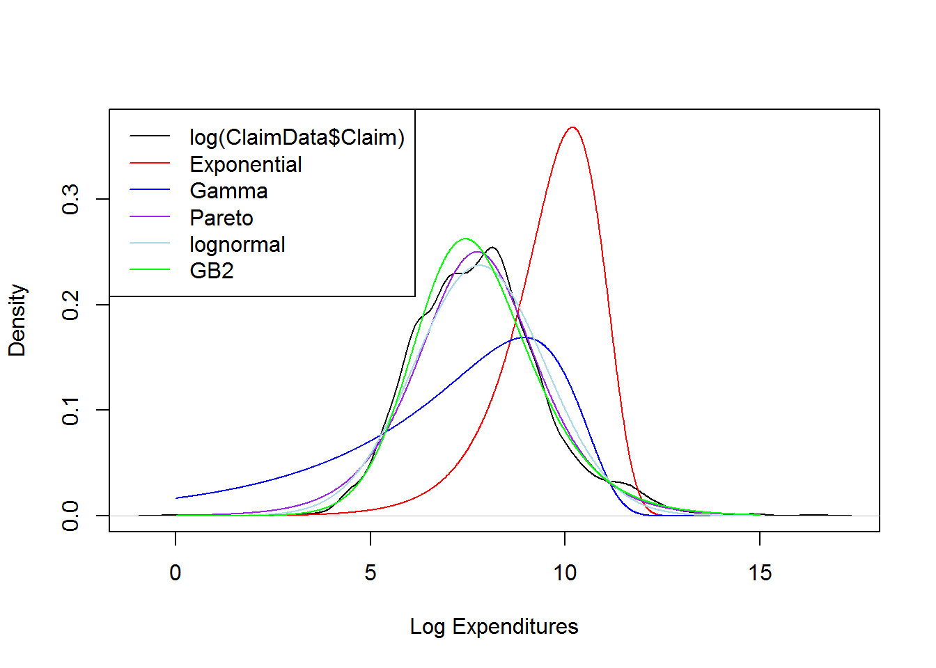

4.4 MLE for grouped data

4.4.1 MLE for grouped data- SOA Exam C # 276

Losses follow the distribution function $F(x)=1-(\theta/x),\quad x>0$ . A sample of 20 losses resulted in the following:

Interval	Number of Losses
(0,10]	9
(10,25]	6
(25,infinity)	5

Calculate the maximum likelihood estimate of $\theta$ .

##Log Likelihood function 
likgrp <- function(theta) {
  loglike <-log(((1-(theta/10))^9)*(((theta/10)-(theta/25))^6)* (((theta/25))^5))
  return(-sum(loglike))
}
#  "optim" is a general purpose minimization function
grplik <- optim(c(1),likgrp,method=c("L-BFGS-B"),hessian=TRUE)
#Estimates - Answer "B" on SoA Problem
grplik$par

## [1] 5.5

#standard error
sqrt(diag(solve(grplik$hessian)))

## [1] 1.11243

#t-statistics
(tstat = grplik$par/sqrt(diag(solve(grplik$hessian))) )

## [1] 4.944132

#Plot of Negative Log-Likelihood function 
vllh = Vectorize(likgrp,"theta")
theta=seq(0,10, by=0.01)
plot(theta, vllh(theta), pch=16, main ="Negative Log-Likelihood function" , cex=.25, 
     xlab=expression(theta), ylab=expression(paste("L(",theta,")")))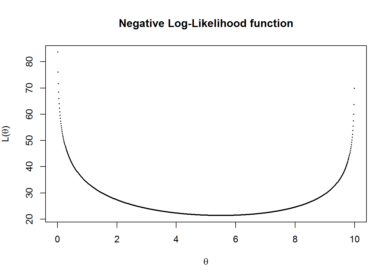

4.5 Nonparametric Inference

4.5.1 Nonparametric Estimation Tools

This section illustrates non-parametric tools including moment estimators, empirical distribution function, quantiles and density estimators.

4.5.1.1 Moment estimators

The $kth$ moment $EX^k$ is estimated by $\frac{1}{n}\sum_{i=1}^{n}X_i^k$ . When $k=1$ then the estimator is called the sample mean.The central moment is defined as $E(X-\mu)^k$ . When $k=2$ , then the central moment is called variance. Below illustrates the mean and variance.

# Start with a simple example of ten points
(xExample = c(10,rep(15,3),20,rep(23,4),30))

##  [1] 10 15 15 15 20 23 23 23 23 30

##summary
summary(xExample) # mean

##    Min. 1st Qu.  Median    Mean 3rd Qu.    Max. 
##    10.0    15.0    21.5    19.7    23.0    30.0

sd(xExample)^2   # variance

## [1] 34.45556

4.5.1.2 Emperical Distribution function

The graph below gives the empirical distribution function xExample dataset.

PercentilesxExample <- ecdf(xExample)

###Empirical Distribution Function
plot(PercentilesxExample, main="",xlab="x")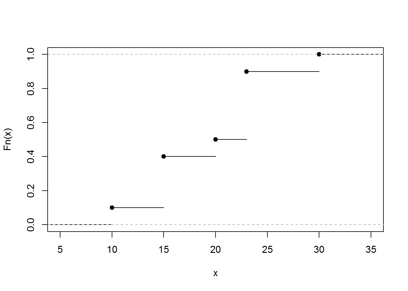

4.5.1.3 Quantiles

The results below gives the quantiles.

##quantiles 
quantile(xExample)

##   0%  25%  50%  75% 100% 
## 10.0 15.0 21.5 23.0 30.0

#quantiles : set you own probabilities
quantile(xExample, probs = seq(0, 1, 0.333333))

##       0% 33.3333% 66.6666% 99.9999% 
## 10.00000 15.00000 23.00000 29.99994

#help(quantile)

4.5.1.4 Density Estimators

The results below gives the density plots using the uniform kernel and triangular kernel.

##density plot 
plot(density(xExample), main="", xlab="x")

plot(density(xExample, bw=.33), main="", xlab="x") # Change the bandwidth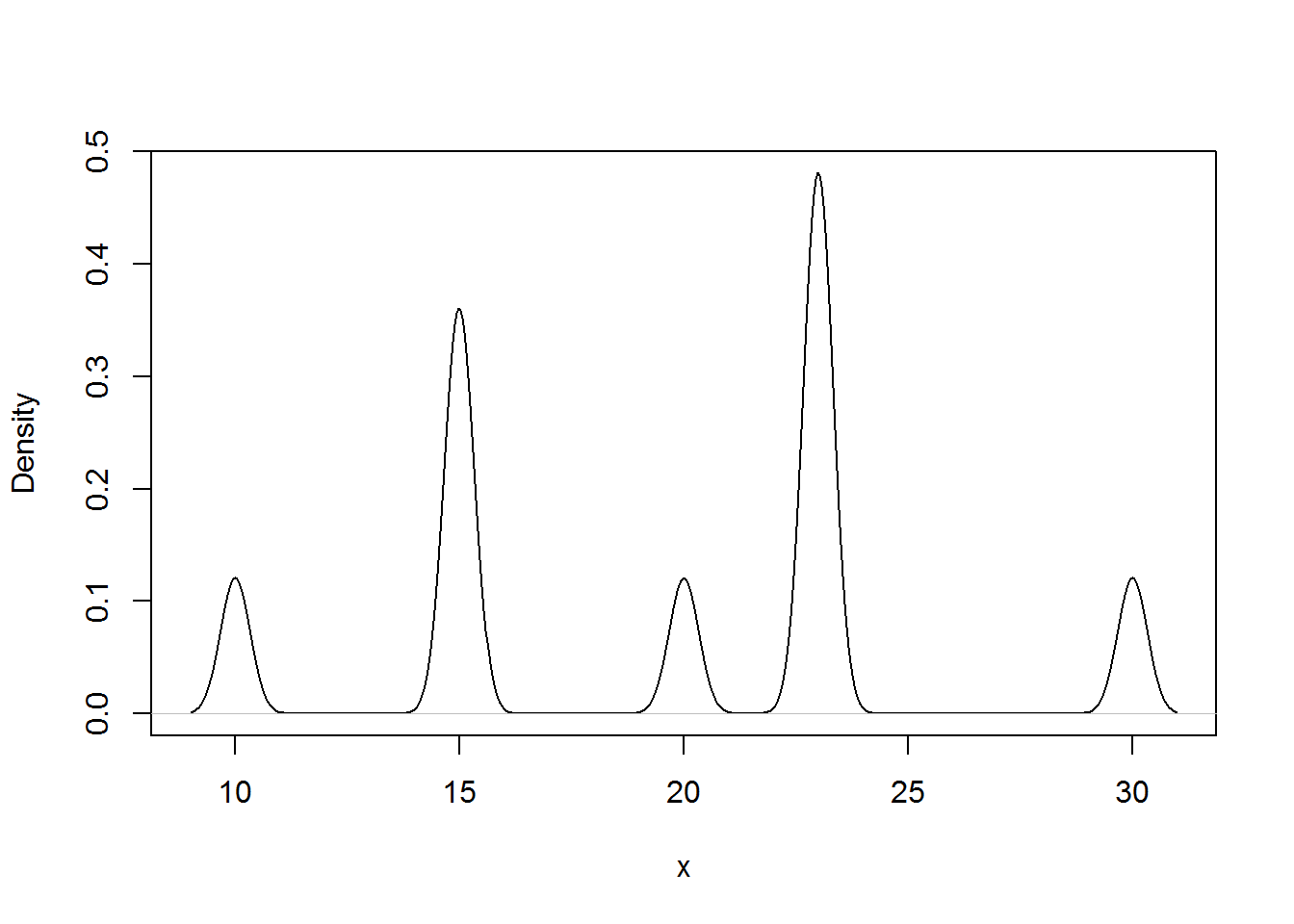

plot(density(xExample, kernel = "triangular"), main="", xlab="x") # Change the kernel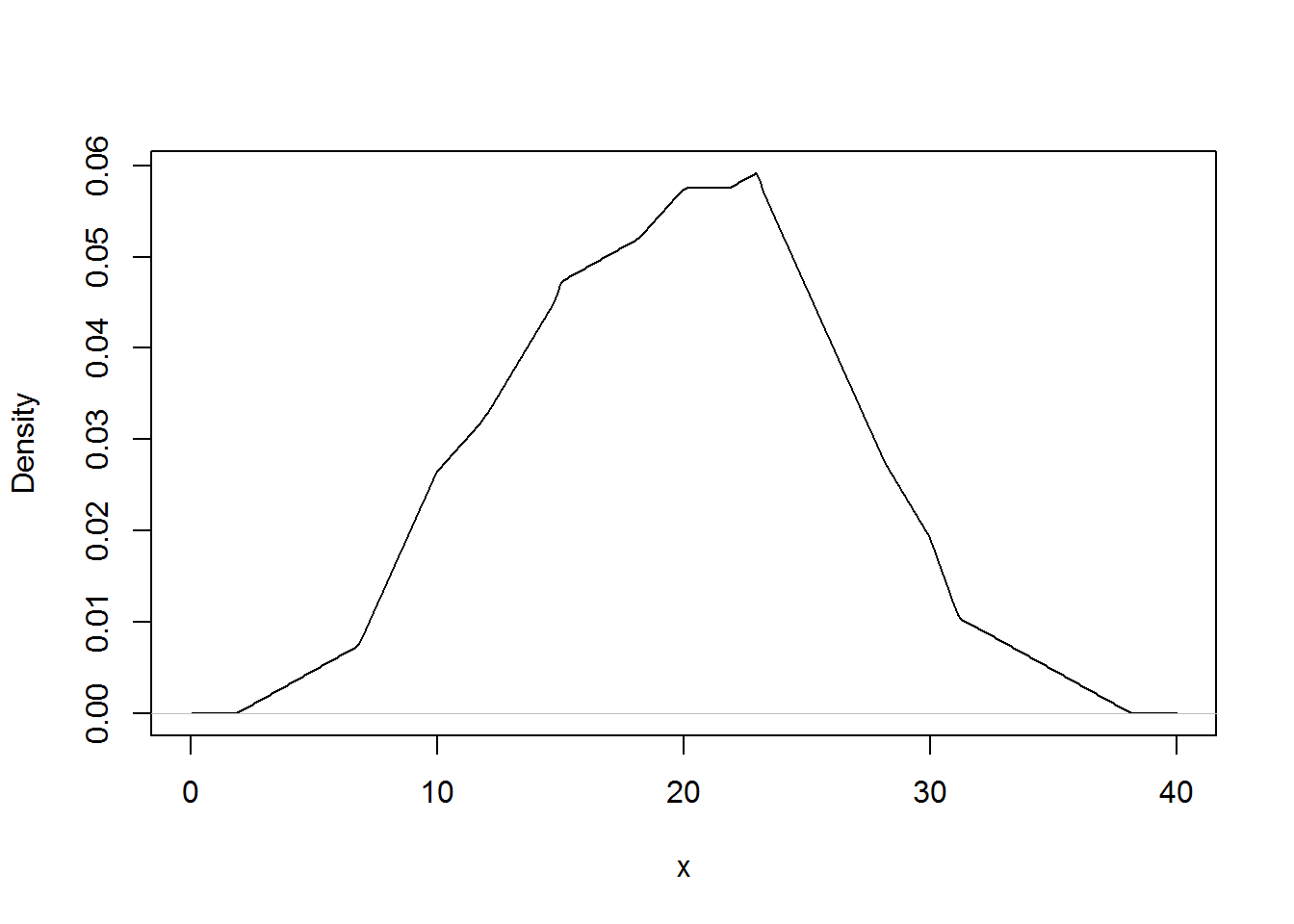

4.5.2 Property Fund Data

This section employs non-parametric estimation tools for model selection for the claims data of the Property Fund.

4.5.2.1 Empirical distribution function of Property fund

The results below gives the empirical distribution function of the claims and claims in logarithmic units.

ClaimLev <- read.csv("DATA/CLAIMLEVEL.csv", header=TRUE); nrow(ClaimLev); # 6258

## [1] 6258

ClaimData<-subset(ClaimLev,Year==2010);     #2010 subset 
##Empirical distribution function of Property fund
par(mfrow=c(1, 2))
Percentiles  <- ecdf(ClaimData$Claim)
LogPercentiles  <- ecdf(log(ClaimData$Claim))
plot(Percentiles,  main="", xlab="Claims")
plot(LogPercentiles, main="", xlab="Logarithmic Claims")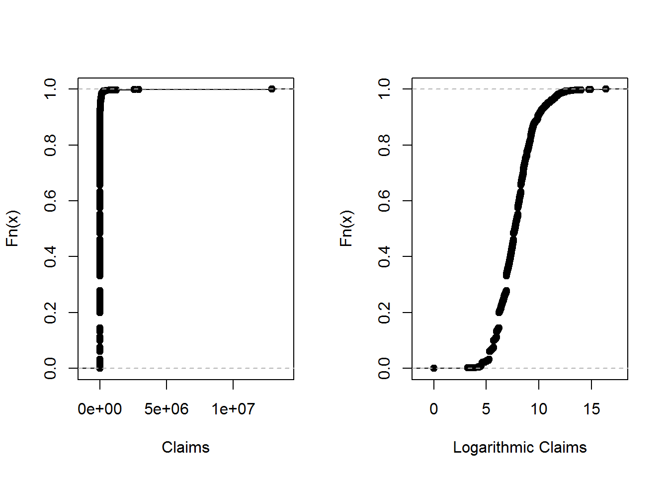

4.5.2.2 Density Comparison

shows a histogram (with shaded gray rectangles) of logarithmic property claims from 2010. The blue thick curve represents a Gaussian kernel density where the bandwidth was selected automatically using an ad hoc rule based on the sample size and volatility of the data.

#Density Comparison
hist(log(ClaimData$Claim), main="", ylim=c(0,.35),xlab="Log Expenditures", freq=FALSE, col="lightgray")
lines(density(log(ClaimData$Claim)), col="blue",lwd=2.5)
lines(density(log(ClaimData$Claim), bw=1), col="green")
lines(density(log(ClaimData$Claim), bw=.1), col="red", lty=3)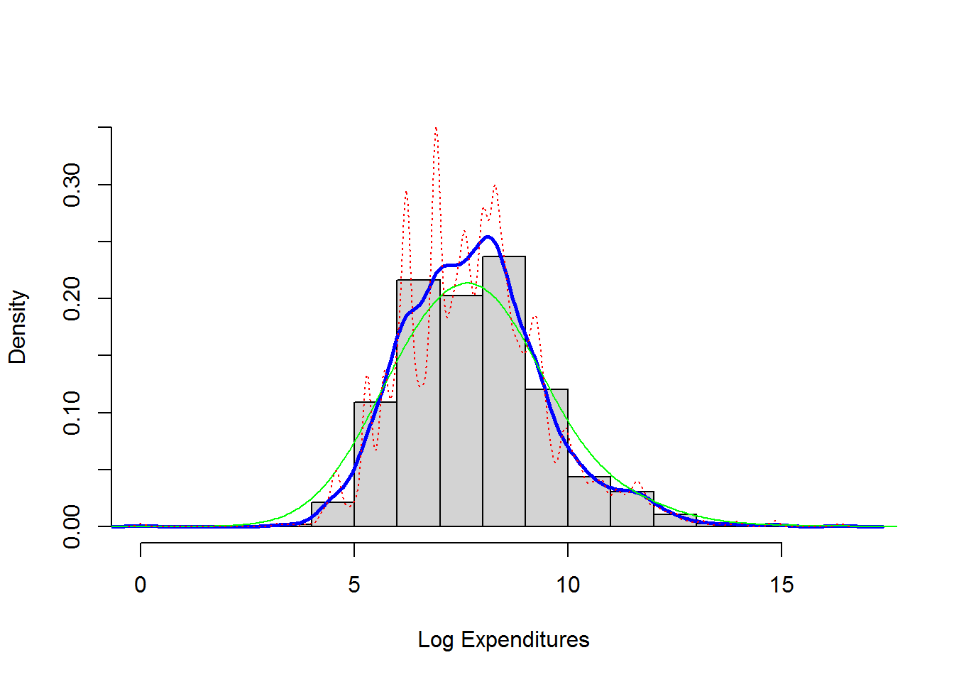

density(log(ClaimData$Claim))$bw   ##default bandwidth

## [1] 0.3255908

4.5.3 Nonparametric Estimation Tools For Model Selection

The results below fits Gamma and Pareto distribution to the claims data

library(MASS)
library(VGAM)
# Inference assuming a gamma distribution
fit.gamma2 <- glm(Claim~1, data=ClaimData,family=Gamma(link=log)) 
summary(fit.gamma2, dispersion = gamma.dispersion(fit.gamma2))

## 
## Call:
## glm(formula = Claim ~ 1, family = Gamma(link = log), data = ClaimData)
## 
## Deviance Residuals: 
##    Min      1Q  Median      3Q     Max  
## -4.287  -2.258  -1.764  -1.178  30.926  
## 
## Coefficients:
##             Estimate Std. Error z value Pr(>|z|)    
## (Intercept) 10.18952    0.04999   203.8   <2e-16 ***
## ---
## Signif. codes:  0 '***' 0.001 '**' 0.01 '*' 0.05 '.' 0.1 ' ' 1
## 
## (Dispersion parameter for Gamma family taken to be 3.441204)
## 
##     Null deviance: 6569.1  on 1376  degrees of freedom
## Residual deviance: 6569.1  on 1376  degrees of freedom
## AIC: 28414
## 
## Number of Fisher Scoring iterations: 14

(theta<-exp(coef(fit.gamma2))*gamma.dispersion(fit.gamma2)) #mu=theta/alpha

## (Intercept) 
##    91613.78

(alpha<-1/gamma.dispersion(fit.gamma2) )

## [1] 0.2905959

#  Inference assuming a Pareto Distribution
fit.pareto <- vglm(Claim ~ 1, paretoII, loc=0, data = ClaimData)
summary(fit.pareto)

## 
## Call:
## vglm(formula = Claim ~ 1, family = paretoII, data = ClaimData, 
##     loc = 0)
## 
## 
## Pearson residuals:
##                 Min      1Q Median     3Q   Max
## loge(scale)  -6.332 -0.8289 0.1875 0.8832 1.174
## loge(shape) -10.638  0.0946 0.4047 0.4842 0.513
## 
## Coefficients: 
##                 Estimate Std. Error z value Pr(>|z|)    
## (Intercept):1  7.7329210  0.0933332  82.853   <2e-16 ***
## (Intercept):2 -0.0008753  0.0538642  -0.016    0.987    
## ---
## Signif. codes:  0 '***' 0.001 '**' 0.01 '*' 0.05 '.' 0.1 ' ' 1
## 
## Number of linear predictors:  2 
## 
## Names of linear predictors: loge(scale), loge(shape)
## 
## Log-likelihood: -13404.64 on 2752 degrees of freedom
## 
## Number of iterations: 5

head(fitted(fit.pareto))

##         [,1]
## [1,] 2285.03
## [2,] 2285.03
## [3,] 2285.03
## [4,] 2285.03
## [5,] 2285.03
## [6,] 2285.03

exp(coef(fit.pareto))

## (Intercept):1 (Intercept):2 
##  2282.2590626     0.9991251

4.5.3.1 Graphical Comparison of Distributions

The graphs below reinforces the technique of overlaying graphs for comparison purposes using both the distribution function and density function. Pareto distribution provides a better fit.

# Plotting the fit using densities (on a logarithmic scale)
# None of these distributions is doing a great job....
x <- seq(0,15,by=0.01)

par(mfrow=c(1, 2))
LogPercentiles  <- ecdf(log(ClaimData$Claim))
plot(LogPercentiles,  main="", xlab="Claims", cex=0.4)
Fgamma_ex = pgamma(exp(x), shape = alpha, scale=theta)
lines(x,Fgamma_ex,col="blue")
Fpareto_ex = pparetoII(exp(x),loc=0,shape = exp(coef(fit.pareto)[2]), scale = exp(coef(fit.pareto)[1]))
lines(x,Fpareto_ex,col="purple")
legend("bottomright", c("log(claims)", "Gamma","Pareto"), lty=1, cex=0.6,col = c("black","blue","purple"))

plot(density(log(ClaimData$Claim)) ,main="", xlab="Log Expenditures")
fgamma_ex = dgamma(exp(x), shape = alpha, scale=theta)*exp(x)
lines(x,fgamma_ex,col="blue")
fpareto_ex = dparetoII(exp(x),loc=0,shape = exp(coef(fit.pareto)[2]), scale = exp(coef(fit.pareto)[1]))*exp(x)
lines(x,fpareto_ex,col="purple")
legend("topright", c("log(claims)", "Gamma","Pareto"), lty=1, cex=0.6,col = c("black","blue","purple"))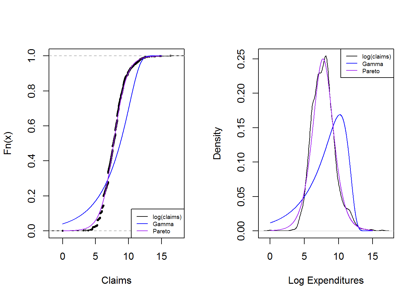

4.5.3.2 P-P plots

shows $pp$ plots for the Property Fund data; the fitted gamma is on the left and the fitted Pareto is on the right. Pareto distribution provides a better fit again

#  PP Plot
par(mfrow=c(1, 2))
Fgamma_ex = pgamma(ClaimData$Claim, shape = alpha, scale=theta)
plot(Percentiles(ClaimData$Claim),Fgamma_ex, xlab="Empirical DF", ylab="Gamma DF",cex=0.4)
abline(0,1)
Fpareto_ex = pparetoII(ClaimData$Claim,loc=0,shape = exp(coef(fit.pareto)[2]), scale = exp(coef(fit.pareto)[1]))
plot(Percentiles(ClaimData$Claim),Fpareto_ex, xlab="Empirical DF", ylab="Pareto DF",cex=0.4)
abline(0,1)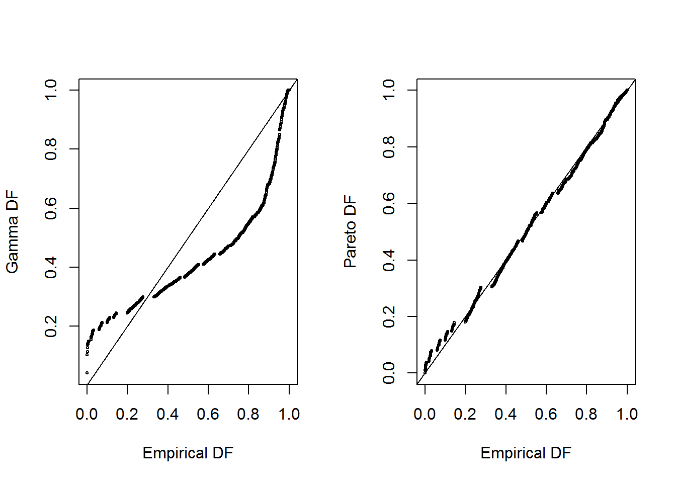

#dev.off()

4.5.3.3 q-q plots

In the graphs below the quantiles are plotted on the original scale in the left-hand panels, on the log scale in the right-hand panel, to allow the analyst to see where a fitted distribution is deficient

##q-q plot
par(mfrow=c(2, 2))
xseq = seq(0.0001, 0.9999, by=1/length(ClaimData$Claim))
empquant = quantile(ClaimData$Claim, xseq)
Gammaquant = qgamma(xseq, shape = alpha, scale=theta)
plot(empquant, Gammaquant, xlab="Empirical Quantile", ylab="Gamma Quantile")
abline(0,1)
plot(log(empquant), log(Gammaquant), xlab="Log Emp Quantile", ylab="Log Gamma Quantile")
abline(0,1)
Paretoquant = qparetoII(xseq,loc=0,shape = exp(coef(fit.pareto)[2]), scale = exp(coef(fit.pareto)[1]))
plot(empquant, Paretoquant, xlab="Empirical Quantile", ylab="Pareto Quantile")
abline(0,1)
plot(log(empquant), log(Paretoquant), xlab="Log Emp Quantile", ylab="Log Pareto Quantile")
abline(0,1)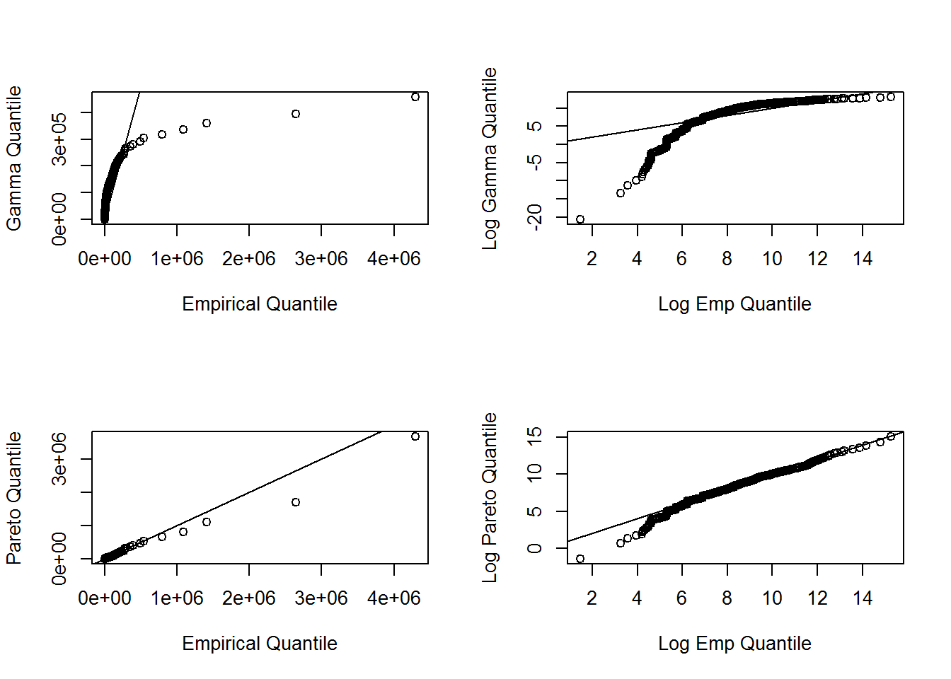

4.5.3.4 Goodness of Fit Statistics

For reporting results, it can be effective to supplement graphical displays with selected statistics that summarize model goodness of fit. The results below provides three commonly used goodness of fit statistics.

library(goftest )
#Kolmogorov-Smirnov # the test statistic is "D"
ks.test(ClaimData$Claim, "pgamma", shape = alpha, scale=theta)

## 
##  One-sample Kolmogorov-Smirnov test
## 
## data:  ClaimData$Claim
## D = 0.26387, p-value < 2.2e-16
## alternative hypothesis: two-sided

ks.test(ClaimData$Claim, "pparetoII",loc=0,shape = exp(coef(fit.pareto)[2]), scale = exp(coef(fit.pareto)[1]))

## 
##  One-sample Kolmogorov-Smirnov test
## 
## data:  ClaimData$Claim
## D = 0.047824, p-value = 0.003677
## alternative hypothesis: two-sided

#Cramer-von Mises # the test statistic is "omega2"
cvm.test(ClaimData$Claim, "pgamma", shape = alpha, scale=theta)

## 
##  Cramer-von Mises test of goodness-of-fit
##  Null hypothesis: Gamma distribution
##  with parameters shape = 0.290595934110839, scale =
##  91613.779421033
## 
## data:  ClaimData$Claim
## omega2 = 33.378, p-value = 2.549e-05

cvm.test(ClaimData$Claim, "pparetoII",loc=0,shape = exp(coef(fit.pareto)[2]), scale = exp(coef(fit.pareto)[1]))

## 
##  Cramer-von Mises test of goodness-of-fit
##  Null hypothesis: distribution 'pparetoII'
##  with parameters shape = 0.999125131378519, scale =
##  2282.25906257586
## 
## data:  ClaimData$Claim
## omega2 = 0.38437, p-value = 0.07947

#Anderson-Darling # the test statistic is "An"
ad.test(ClaimData$Claim, "pgamma", shape = alpha, scale=theta)

## 
##  Anderson-Darling test of goodness-of-fit
##  Null hypothesis: Gamma distribution
##  with parameters shape = 0.290595934110839, scale =
##  91613.779421033
## 
## data:  ClaimData$Claim
## An = Inf, p-value = 4.357e-07

ad.test(ClaimData$Claim, "pparetoII",loc=0,shape = exp(coef(fit.pareto)[2]), scale = exp(coef(fit.pareto)[1]))

## 
##  Anderson-Darling test of goodness-of-fit
##  Null hypothesis: distribution 'pparetoII'
##  with parameters shape = 0.999125131378519, scale =
##  2282.25906257586
## 
## data:  ClaimData$Claim
## An = 4.1264, p-value = 0.007567